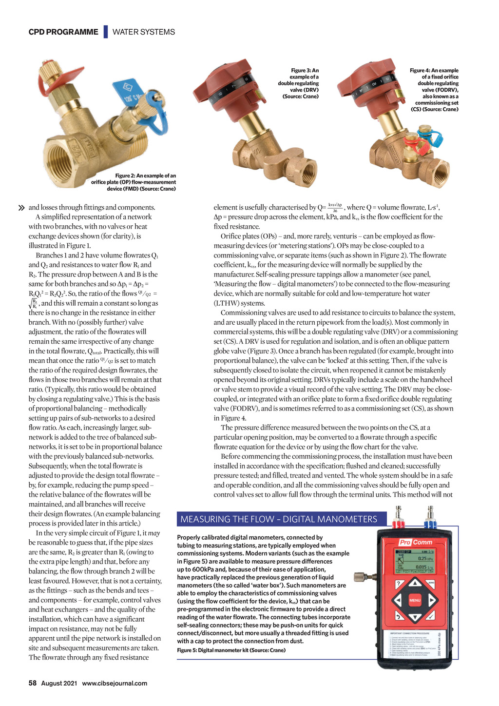


CPD PROGRAMME | WATER SYSTEMS Figure 3: An example of a Figure 4: An example Figure 2: An example of an and losses through fittings and components. A simplified representation of a network with two branches, with no valves or heat exchange devices shown (for clarity), is illustrated in Figure 1. Branches 1 and 2 have volume flowrates Q1 and Q2 and resistances to water flow R1 and R2. The pressure drop between A and B is the same for both branches and so p1 = p2 = R1Q12 = R2Q22. So, the ratio of the flows Q1Q2 = , and this will remain a constant so long as there is no change in the resistance in either branch. With no (possibly further) valve adjustment, the ratio of the flowrates will remain the same irrespective of any change in the total flowrate, Qtotal. Practically, this will mean that once the ratio Q1Q2 is set to match the ratio of the required design flowrates, the flows in those two branches will remain at that ratio. (Typically, this ratio would be obtained by closing a regulating valve.) This is the basis of proportional balancing methodically setting up pairs of sub-networks to a desired flow ratio. As each, increasingly larger, subnetwork is added to the tree of balanced subnetworks, it is set to be in proportional balance with the previously balanced sub-networks. Subsequently, when the total flowrate is adjusted to provide the design total flowrate by, for example, reducing the pump speed the relative balance of the flowrates will be maintained, and all branches will receive their design flowrates. (An example balancing process is provided later in this article.) In the very simple circuit of Figure 1, it may be reasonable to guess that, if the pipe sizes are the same, R2 is greater than R1 (owing to the extra pipe length) and that, before any balancing, the flow through branch 2 will be least favoured. However, that is not a certainty, as the fittings such as the bends and tees and components for example, control valves and heat exchangers and the quality of the installation, which can have a significant impact on resistance, may not be fully apparent until the pipe network is installed on site and subsequent measurements are taken. The flowrate through any fixed resistance element is usefully characterised by Q= kvs36 p , where Q = volume flowrate, L.s-1, p = pressure drop across the element, kPa, and kvs is the flow coefficient for the fixed resistance. Orifice plates (OPs) and, more rarely, venturis can be employed as flowmeasuring devices (or metering stations). OPs may be close-coupled to a commissioning valve, or separate items (such as shown in Figure 2). The flowrate coefficient, kvs, for the measuring device will normally be supplied by the manufacturer. Self-sealing pressure tappings allow a manometer (see panel, Measuring the flow digital manometers) to be connected to the flow-measuring device, which are normally suitable for cold and low-temperature hot water (LTHW) systems. Commissioning valves are used to add resistance to circuits to balance the system, and are usually placed in the return pipework from the load(s). Most commonly in commercial systems, this will be a double regulating valve (DRV) or a commissioning set (CS). A DRV is used for regulation and isolation, and is often an oblique pattern globe valve (Figure 3). Once a branch has been regulated (for example, brought into proportional balance), the valve can be locked at this setting. Then, if the valve is subsequently closed to isolate the circuit, when reopened it cannot be mistakenly opened beyond its original setting. DRVs typically include a scale on the handwheel or valve stem to provide a visual record of the valve setting. The DRV may be closecoupled, or integrated with an orifice plate to form a fixed orifice double regulating valve (FODRV), and is sometimes referred to as a commissioning set (CS), as shown in Figure 4. The pressure difference measured between the two points on the CS, at a particular opening position, may be converted to a flowrate through a specific flowrate equation for the device or by using the flow chart for the valve. Before commencing the commissioning process, the installation must have been installed in accordance with the specification; flushed and cleaned; successfully pressure tested; and filled, treated and vented. The whole system should be in a safe and operable condition, and all the commissioning valves should be fully open and control valves set to allow full flow through the terminal units. This method will not MEASURING THE FLOW DIGITAL MANOMETERS Properly calibrated digital manometers, connected by tubing to measuring stations, are typically employed when commissioning systems. Modern variants (such as the example in Figure 5) are available to measure pressure differences up to 600kPa and, because of their ease of application, have practically replaced the previous generation of liquid manometers (the so called water box). Such manometers are able to employ the characteristics of commissioning valves vs) that can be self-sealing connectors; these may be push-on units for quick with a cap to protect the connection from dust. 58 August 2021 www.cibsejournal.com CIBSE Aug 21 pp57-60 CPD 183.indd 58 23/07/2021 12:19